7.7 Plotting Taylor's Series

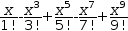
This example shows how the limit value in a summation can be bound to a real definition. The Taylor series for sin x is given by ∑0, 4, -1^n⋅x^(2⋅n+1)÷(2⋅n+1) !ⅆn. Distributing and simplifying gives x÷1 !-x^3÷3 !+x^5÷5 !-x^7÷7 !+x^9÷9 !.

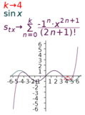
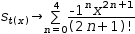
How close to sin x is the 5-term series expansion? To answer this, plot both the series and sin x. (You'll have to plot the summation using the function definition s_t(x)→∑0, 4, -1^n⋅x^(2⋅n+1)÷(2⋅n+1) !ⅆn.) The initial plot displays x and y values in the unit range and shows the two functions have identical values, but when the x axis is extended past ±5, the values of the 5-term Taylor series begin to differ.

To investigate further the effect of changing the limit of the summation, replace it with a variable that is defined elsewhere on the display. Then plot both the series function and the variable.

These functions need to be added to the plotter:

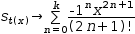
• s_t(x)→∑0, k, -1^n⋅x^(2⋅n+1)÷(2⋅n+1) !ⅆn
• sin x
• k→4

The variable definition k→4 adjusts the number of terms in the summation. With the adjuster set to 4, the plot should look like Figure 7.13.